09.07.2026
From World Models to Physical AI: Building Test Data for AIDC Inspection with NVIDIA Cosmos 3
What You Will Learn
- How world models fill the test-data gap for Physical AI
- How to generate video and audio in one pass with Cosmos 3, and how the prompts for the three sample groups are written
- How to connect data generation, visual interpretation and audio analysis into one pipeline while keeping the answer key away from the interpretation side
1. Test Data Comes First, Inspection Results Second
Before Physical AI can move into AIDC inspection, and before we ask whether a model answers correctly, there has to be enough data to test against repeatedly. Obvious anomalies — smoke, standing water, a rack on fire — are not hard to demonstrate. The awkward cases are the unremarkable state changes: one amber LED in a row of green, a missing blanking panel, a rack door that never quite latched, or a single line of warning text on a screen.
Material like that is hard to collect systematically. Cosmos 3 can generate a specified scenario up front, filling in the rare or hard-to-stage test cases. So we built a reusable set of synthetic samples to serve as a screening pass ahead of formal on-site testing.
2. Building Samples with Preset Labels from a World Model
We deployed the NVIDIA Cosmos3-Nano Generator as an inference service, producing video and audio within the same inference pass rather than dubbing an audio track afterwards. That lets us try to build samples where the picture is normal but the sound is not, through the prompt alone, and then check by hand whether the generated content matches the setup.
On that basis we generated 170 data center inspection videos, in three groups:
- Baseline group: 50 normal videos and 50 with clearly visible anomalies, such as smoke, fire, water ingress, arcing and toppled racks
- Subtle group: 35 videos depicting subtle anomalies, plus 15 normal clips
- Audio group: 20 videos with a normal picture but anomalous sound; for evaluation we drew a further 65 videos from the first two groups whose prompts specified no abnormal sound, and used their ambient audio as negative samples
2.1 Video and Audio in One Pass
In this pipeline we use the Cosmos3-Nano Generator to produce video from a prompt, and the Cosmos3-Nano Reasoner for visual interpretation. The generation side has a single interface: send in a prompt, get back a 720p clip of about 2.5 seconds with the audio track already in it.
All 170 clips share one set of generation parameters; only the prompt and the random seed change, so there are no other variables to account for when comparing clips later.
2.2 How the Prompts Are Written
Each clip's prompt has two parts: a scene description followed by a sound description. The three groups are written differently, and the examples below show only the scene part.
The baseline group describes either a normal data hall or a clearly visible anomaly. There are 25 prompts for each class, each run with 2 random seeds, giving 50 clips per class. The scene part of an anomaly prompt looks like this:
A swollen leaking UPS battery venting fumes in the battery room.
The subtle group covers the kind of anomaly described in section 1: a single amber LED, a door not fully latched, a missing blanking panel, plus dust on an intake filter, condensation and a tool left behind. Another 15 clips are written as normal scenes so this group has negatives too.
The audio group describes a normal scene and puts a fault sound in the sound description. The fault sounds cover low-frequency mechanical sources such as bearings, transformers and relays, as well as high-pitched squeals, broadband hiss and impulses.
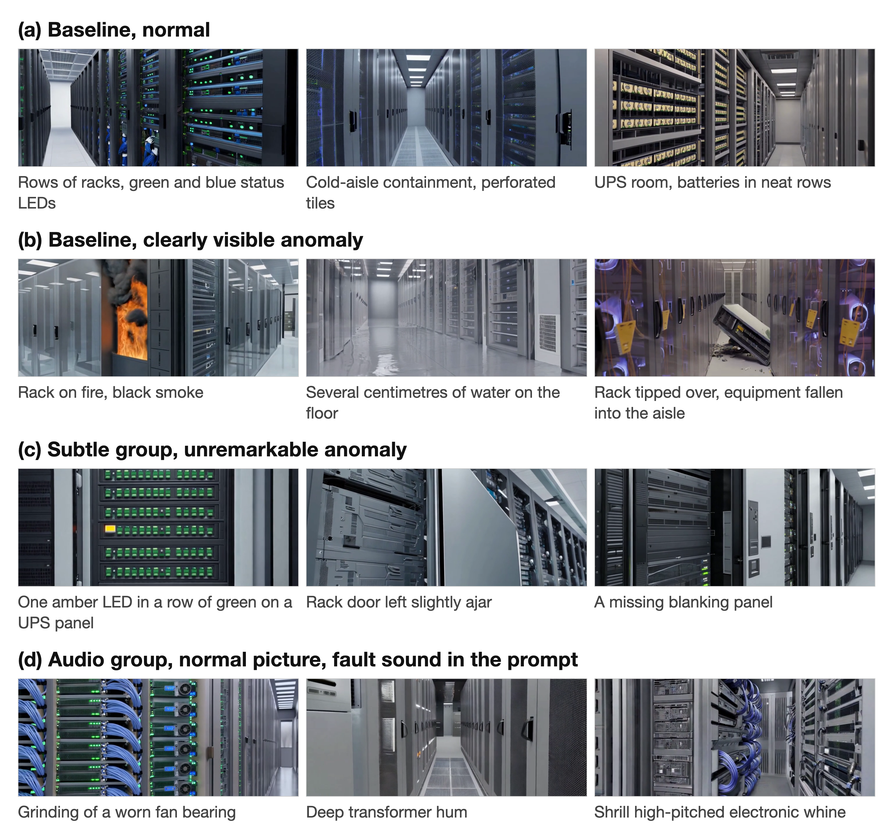
The frames above are cropped from the review video with the overlay bars removed. The subtle row explains what makes this data hard: the amber LED, the door gap and the missing blanking panel are obvious to a human at a glance, yet each occupies a tiny fraction of the frame.
The normal and anomalous labels are taken from the prompts. They represent the scenario a given video was meant to depict, and are not equivalent to ground truth measured in a real facility. Below we call them scenario labels.
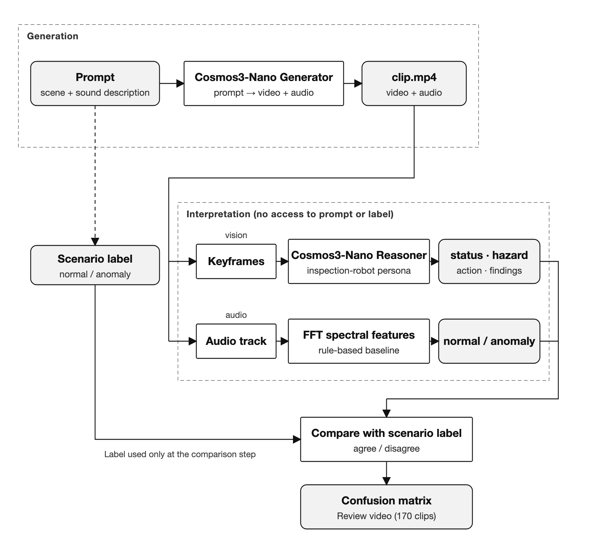
Generation and interpretation stay separate. Prompts go to the Generator only; at interpretation time the Reasoner sees just the picture, and the FFT rules analyse just the waveform. Neither side has access to the prompt. The numbers below reflect only how this pipeline behaves on synthetic data.
3. From Generation to Interpretation
The pipeline has two stages, generation and interpretation, joined only by the video file itself; the scenario label is held back until the final comparison step. Once a video reaches the interpretation side, vision and audio are handled separately.
3.1 Visual Interpretation
Visual interpretation runs only on the baseline and subtle groups; the 20 audio-group clips are not counted in the Reasoner scoring and only go through the audio interpretation described in 3.2. On the vision side we extract keyframes from the video and pass them to the Cosmos3-Nano Reasoner. We give the Reasoner an inspection-robot persona and ask it to return four fields in a fixed format: status is normal or anomaly, hazard is the hazard category, action is the recommended action, and findings is what it sees in the picture.
Our scenario labels are binary, normal or anomaly, so scoring compares status only. Hazard and action have no label to compare against; they are overlaid on the review video and checked by eye.
3.2 Audio Interpretation
On the audio side we extract the track and first build a rule-based anomaly-detection baseline on FFT spectral features: a handful of features such as crest factor, peak frequency and high-frequency content, sorted into normal or anomaly with threshold rules, with no learned model. The point of this step is to confirm that the whole multimodal pipeline runs end to end; the interpretation module can be replaced or upgraded later.
The thresholds were calibrated on both classes together: the fault sounds of the 20 audio-group clips, and the ambient audio of the 65 clips from the first two groups whose prompts specified no abnormal sound, keeping only the features that separate the two.
3.3 Comparison, Scoring and Review
Once interpretation is done, we match each clip's verdict against its scenario label and arrange the counts in a confusion matrix. The numbers that come out measure agreement between the verdicts and the scenario labels, not detection accuracy in a real facility.
The 100 baseline clips contain 50 normal and 50 clearly anomalous videos; for 96 of them the Reasoner verdict agreed with the scenario label set at generation time (96%). This figure reflects end-to-end consistency on this batch of synthetic data.
| Reasoner verdict: normal | Reasoner verdict: anomaly | |
|---|---|---|
| Scenario label: normal (50) | 50 | 0 |
| Scenario label: anomaly (50) | 4 | 46 |
All 4 disagreements fall in the half labelled anomalous. This post uses the 100 baseline clips to validate the end-to-end pipeline; the subtle and audio groups mainly serve to build stress-test data for later work, and we do not treat their results as model performance figures here.
Each video is overlaid with its prompt, verdict and scenario label, keeps the audio as generated, and the whole set is then composited into one review video of 7 minutes 12 seconds. This overlay format reads more directly than a statistics table on its own, and it makes it straightforward to walk back through the clips one by one and check whether the generated content actually matches the prompt.
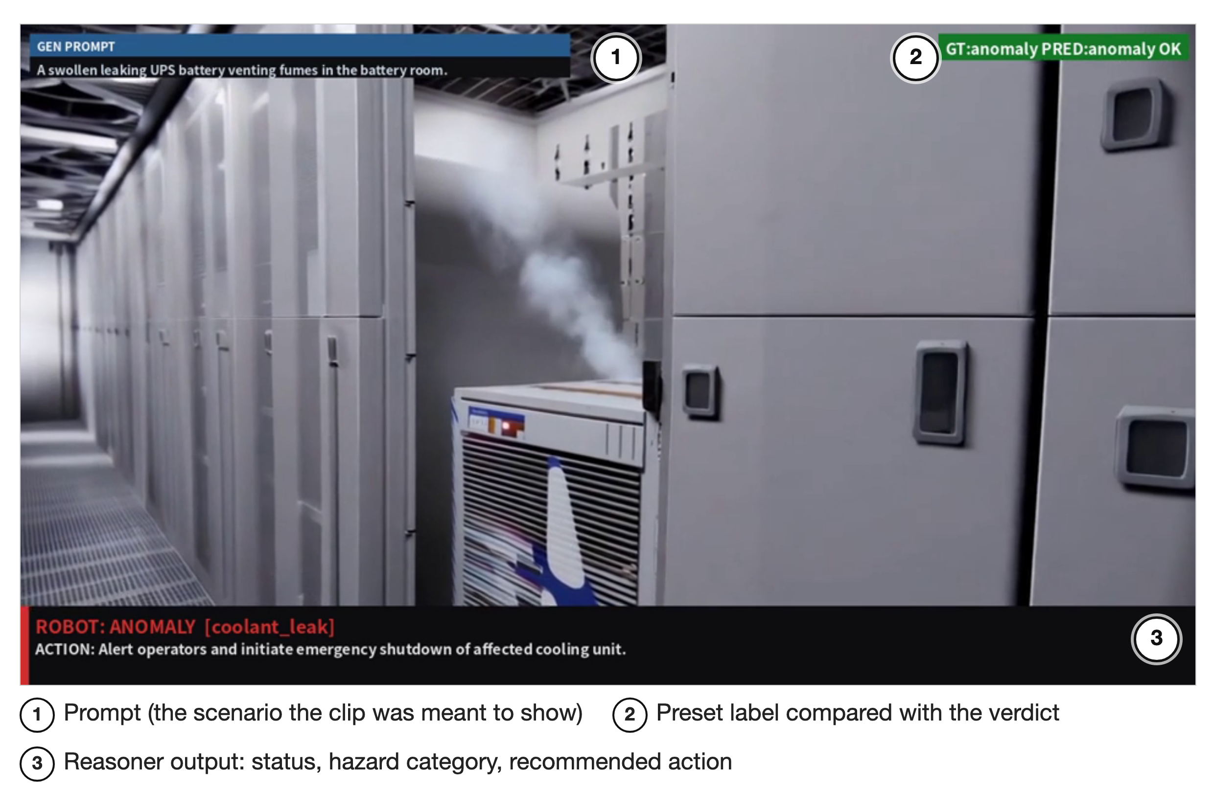
This frame also shows why hazard needs a human eye. The prompt describes a swollen UPS battery leaking and venting fumes, but the unit smoking in the frame looks more like a cooling unit; the Reasoner judged it anomalous and labelled the hazard coolant_leak. The normal-or-anomaly verdict is right, the category does not match the prompt, and the cause may sit on the generation side rather than the reasoning side. That is exactly why each clip needs to be checked against its prompt. The GT in the top right corner means the scenario label, not ground truth measured on site.
4. What This Pipeline Is Good For
The point of this exercise is not to replace field data with synthetic data, but to first organise rare, hard-to-collect scenarios into a test set that can be run repeatedly. The division of labour is clear: the Generator builds the test world, the prompt defines the intended scenario, a human confirms generation fidelity, the Reasoner handles visual understanding, the FFT rules serve as the audio anomaly baseline, and the fixed dataset is kept for later regression tests. Prompts control the scenario and the anomaly type, and the same interpretation pipeline can be re-run at will, which suits quick before-and-after comparisons whenever a model or a rule changes.
Synthetic data still has clear limits. A prompt that specifies an anomaly is no guarantee that the generated video depicts it faithfully; every sample needs human review, and any formal evaluation has to bring in real facility footage and recordings as well. In addition, visual interpretation currently works from sampled keyframes, so an anomaly that appears only briefly, or falls between sampling points, can be missed; errors of that kind need to be analysed separately from the Reasoner's own misreadings. When we look at misses later, there are three layers to separate: whether the Generator actually produced the anomaly, whether the keyframes caught it, and whether the Reasoner understood the picture. Not every error belongs to the Reasoner.
Closing
This exercise produced 170 audio-video samples, and connected scene generation, visual interpretation, audio analysis and result aggregation into one repeatable pipeline. When a model or an interpretation rule is updated, the same batch of data can be run again without preparing material from scratch each time.
For AIDC inspection we are keeping world models in a clearly bounded role for now: build the test scenarios that are hard to collect, use them to check the pipeline and surface problems, then move on to validation in a real facility. Synthetic data does not replace field data, but it does give Physical AI one more controlled test before deployment.